A little bit theory on unconstrained optimization

In unconstrained optimization one wishes to minimize or maximize a given function $f$ , the so called objective function, without further constraints. We stick here on minimization, maximization may be done then by reversing the sign of $f$. Without some additional assumptions the task might not be solvable at all, hence we present here some (not too hard) restrictions on $f$ which give us a well defined environment to work in.

1. The domain $D$ of $f$ is open in $R^n$.
2. There is a $x^0\hspace{0.5em}\in \hspace{0.5em}D$ such that the level set
   

   ${\displaystyle L(f;x^0)=\{x\hspace{0.5em}\in \hspace{0.5em}D\hspace{0.5em}:\hspace{0.5em}f(x)\hspace{0.5em}\le \hspace{0.5em}f(x^0)\}}$

   
   is closed and bounded in $R^n$ (i.e. compact).
3. $f$ is two times continuously differentiable on an open neighborhood of $L(f;x^0)$.

>From this the following facts follow easily using a little calculus:

1. There exists a $x^{*}$ in $L(f;x^0)$ such that
   

   ${\displaystyle f(x^{*})\hspace{0.5em}\le \hspace{0.5em}f(x)\mathrm{\hspace{1em}\hspace{1em}\hspace{1em}}\forall \hspace{0.5em}x\in D\mathrm{\hspace{1em}\hspace{1em}\hspace{1em}}\text{(the global minimizer)}}$

   
   
2. If $x^{*}$ is a local minimizer in $L(f;x^0)$ , i.e.
   

   ${\displaystyle f(x^{*})\hspace{0.5em}\le \hspace{0.5em}f(x)\mathrm{\hspace{1em}\hspace{1em}\hspace{1em}}\forall \hspace{0.5em}x\in D\cap \{x:||x-x^{*}||\hspace{0.5em}\le \hspace{0.5em}\delta \}}$

   
   for some $\delta >0$ , then there holds
   

   ${\displaystyle \nabla f(x^{*})\hspace{0.5em}=\hspace{0.5em}0\hspace{0.5em}\text{and}\hspace{0.5em}{\nabla }^{2}f(x^{*})\hspace{0.5em}\text{is positive semidefinite,}}$

   
   the so called necessary first and second order optimality conditions.
3. If $\nabla f(x^{*})\hspace{0.5em}=\hspace{0.5em}0$ and ${\nabla }^{2}f(x^{*})$ is positive definite, then $x^{*}$ is a strict local minimzer of $f$, i.e.
   

   ${\displaystyle f(x^{*})\hspace{0.5em}<\hspace{0.5em}f(x)\mathrm{\hspace{1em}\hspace{1em}\hspace{1em}}\forall \hspace{0.5em}x\in D\cap \{x:0\hspace{0.5em}<\hspace{0.5em}||x-x^{*}||\hspace{0.5em}\le \delta \}}$

   
   for some $\delta >0$. A sufficient strict local optimality condition.

With the exception of the Newton-minimizer in this chapter all the codes restrict themselves to find a point satisfying the first order necessary condition

${\displaystyle \nabla f(x^{*})\hspace{0.5em}=\hspace{0.5em}0\hspace{0.5em}.}$

Silently one hopes that from the fact that by construction of the methods there holds a strict monotonic decrease of some associated sequence of function values if might follow, that the limit point one obtains will be a strict local minimizer. There exist methods which indeed guarantee to obtain the global minimizer, but these are of a completely different structure from those presented here. The general structure of most of the methods in this chapter is as follows: Given $x^0$ (hopefully as assumed above) one computes a sequence $\{x^k\}$ from

${\displaystyle x^{k+1}\hspace{0.5em}=\hspace{0.5em}{x}^k-{\sigma }_k{d}^k}$

where $d^k$ is strictly gradient related, this means

${\displaystyle {\gamma }_1||\nabla f(x^k)||\hspace{0.5em}\le \hspace{0.5em}||d^k||\hspace{0.5em}\le \hspace{0.5em}{\gamma }_2||\nabla f(x^k)||}$

and

${\displaystyle \frac{\nabla f(x^k{)}^T{d}^k}{||d^k||||\nabla f(x^k)||}\hspace{0.5em}\ge \hspace{0.5em}{\gamma }_3\hspace{0.5em}>\hspace{0.5em}0}$

for some constants ${\gamma }_1,\hspace{0.5em}{\gamma }_2,\hspace{0.5em}{\gamma }_3\hspace{0.5em}>\hspace{0.5em}0$ which are implicit in the construction of $d^k$, not necessarily explicitly known. In words: the direction of change is of comparable length with the current gradient and has an angle with it, which is bounded away from $\pi /2$. Mostly this property is obtained by choosing $d^k$ as the solution of a linear system

${\displaystyle A_k{d}^k=\nabla f(x^k)}$

with a sequence of matrices $A_k$, whose eigenvalues are bounded from below by a positive constant and bounded from above too. Such a sequence of matrices is called uniformly positive definite. The stepsize ${\sigma }_k$ is computed such that it satisfies the so called principle of sufficient decrease:

${\displaystyle f(x^k)-f(x^k-{\sigma }_k{d}^k)\hspace{0.5em}\ge \hspace{0.5em}{\gamma }_4{\sigma }_k\nabla f(x^k{)}^T{d}^k}$

and

${\displaystyle {\sigma }_k\hspace{0.5em}\ge \hspace{0.5em}{\gamma }_5\frac{\nabla f(x^k{)}^T{d}^k}{||d^k|{|}^2}}$

${\gamma }_4$ is an explicitly known constant, provided by the user (in the codes in this chapter it is the parameter $\delta$) and should be chosen less than 0.5 for efficiency reasons. The existence of ${\gamma }_5$ is assured by the assumptions on $f$ and the construction of $\sigma$, but it is usually unknown. Inserting all the above one gets

${\displaystyle f(x^k)-f(x^{k+1})\hspace{0.5em}\ge \hspace{0.5em}{\gamma }_4{\gamma }_5{\gamma }_3^2||\nabla f(x^k)|{|}^2\hspace{0.5em}\ge \hspace{0.5em}0}$

and from the boundedness of $f$ from below that

${\displaystyle \nabla f(x^k)\hspace{0.5em}\to \hspace{0.5em}0}$

and from this that every limit point of $\{x^k\}$ is a first order necessary point. Clearly $\{x^k\}$ has limit points. One also gets

${\displaystyle d^k\hspace{0.5em}\to \hspace{0.5em}0\hspace{0.5em}.}$

Hence if $\{{\sigma }_k\}$ is also bounded one gets

${\displaystyle x^k-x^{k+1}\hspace{0.5em}\to \hspace{0.5em}0}$

and if $f$ has only finitely many stationary points then the whole sequence $\{x^k\}$ must converge to one of these. This is what a user hopes for: the code delivers a sequence such that termination with

${\displaystyle ||\nabla f(x^k)||\hspace{0.5em}\le \hspace{0.5em}ϵ\hspace{0.5em}\text{or}\hspace{0.5em}||x^k-x^{k+1}||\hspace{0.5em}\le \hspace{0.5em}ϵ}$

delivers him a result "near" a true solution. Up to a second order term the error $x^{*}-x^k$ will be

${\displaystyle ({\nabla }^{2}f(x^k{))}^{-1}\nabla f(x^k)}$

hence if the method delivers a $d^k$ such that

${\displaystyle \frac{||{\nabla }^{2}f(x^k)-A_k)d^k||}{||d^k||}\hspace{0.5em}\to \hspace{0.5em}0}$

(the so called Broyden-Dennis-Morè condition) then termination on grounds of a small difference in $x^k$ will also be a reliable one. We mentioned the construction of $d^k$ above already. The codes in use satisfy this, sometimes with $A_k$ constructed explicitly, sometimes with $A_k$ existing but not known explicitly. We now turn to the computation of the stepsize ${\sigma }_k$. Two methods are in use here: The simplest one is known as backtracking or Goldstein-Armijo descent test and works as follows: Given a strictly gradient related direction $d^k$ choose some initial stepsize ${\sigma }_{0,k}$ less than some universal constant ${\gamma }_0$ (often =1). Then take as ${\sigma }_k$ the largest value ${\beta }^j{\sigma }_{0,k}$ which satisfies

${\displaystyle f(x^k)-f(x^k-{\beta }^j{\sigma }_{0,k}{d}^k)\hspace{0.5em}\ge \hspace{0.5em}\delta {\beta }^j{\sigma }_{0,k}\nabla f(x^k{)}^T{d}^k}$

with a parameter $0\hspace{0.5em}<\hspace{0.5em}\beta \hspace{0.5em}<\hspace{0.5em}1$, (often $\beta =1/2$) and $0\hspace{0.5em}<\hspace{0.5em}\delta \hspace{0.5em}<\hspace{0.5em}1$, preferably $0\hspace{0.5em}<\hspace{0.5em}\delta \hspace{0.5em}<\hspace{0.5em}1/2$. The efficiency of this method depends on the proper choice of ${\sigma }_{0,k}$. For example the minimizer of the parabola interpolating the values

${\displaystyle p(0),\hspace{0.5em}p(1),\hspace{0.5em}p\text{'}(0),\hspace{0.5em}\text{with}\hspace{0.5em}p(s)\hspace{0.5em}=\hspace{0.5em}f(x^k-s{d}^k)}$

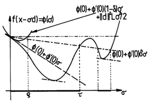
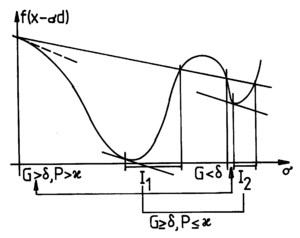
is often useful. The picture above shows you the graph of a function, its tangent line at $\sigma \hspace{0.5em}=\hspace{0.5em}0$, the "Armijo line" used in the test, two intervals of admissible stepsizes and the local upper bound on $f$, a parabola in which the upper bound $L$ for $||{\nabla }^{2}f(x)||$ on the $L(f;x^0)$ enters. This parabola is used to prove that there always are stepsizes satisfying the principle of sufficient decrease. The drawback of dependency on ${\sigma }_{0,k}$ is avoided by the so called Powell-Wolfe stepsize which is independent of such: here a stepsize ${\sigma }_k$ is computed such that

${\displaystyle \begin{array}{ccc}\multicolumn{1}{c}{f(x^k)-f(x^k-\sigma d^k)\hspace{0.5em}}& \ge \hfill & \hspace{0.5em}\delta \sigma \nabla f(x^k{)}^T{d}^k\hfill \\ \multicolumn{1}{c}{}& \text{and}\hfill & \hfill \\ \multicolumn{1}{c}{\nabla f(x^k-\sigma d^k{)}^T{d}^k\hspace{0.5em}}& \le \hfill & \hspace{0.5em}\kappa \nabla f(x^k{)}^T{d}^k\hfill \end{array}}$

with $0\hspace{0.5em}<\hspace{0.5em}\delta \hspace{0.5em}<\hspace{0.5em}\kappa <\hspace{0.5em}1$. Sometimes the strong Powell-Wolfe conditions are used, where on the left hand side of the second inequality the absolute sign is used. This means that a local first order stationary point on the search line is required. The picture above shows you a graph of a function and two admissible intervals of stepsizes. Observe, that due to the second condition, in contrast to the backtracking scheme arbitrarily small stepsizes or not admissible here. If the strong conditions would be used too, then only two small intervals around the two local minimizers would remain as admissible.

---

File translated from T_EX by T_TM Unregistered, version 4.03.
On 16 Jun 2016, 18:14.