Nelder-Mead: mathematical correct version

Directly to the input form

• The method of Nelder and Mead (British Computer Journal 7, 1965, 308-313) is a so called ''derivative free'' method for minimizing functions, using function values only. Although mathematically incorrect (as shown by McKinnon in SIOPT 1998), it is the most used from practitioners. This may be due to the fact that it is of great simplicity and mostly produces good solutions at least in low dimensions. There exist a lot of modifications of the original method, some aiming in making it provably mathematically correct. These modifications typically use ingredients of other methods, like grid search or the principle of sufficient decrease. Here we use a modification of A. Witzel (PhD dissertation, TUD ,2008) which only uses minimal changes to the original method.
• In each step of the method one has a simplex in Rⁿ (the convex hull of n+1 affinely independent points, for n=2 a triangle) and the function values at the vertices xⁱ, i=0,...,n, i.e. f(xⁱ) . The current step aims in computing a new simplex with decreased worst (largest) function value. This is done by applying a set of replacement rules for the vertices. For a simplex with vertices xⁱ, i=0,...,n define
  
  1. f_h = max { f(x^j): j=0,...,n }, the largest function value
     
  2. H = { i: f(xⁱ) >= f_h - ε_f*ρ }, the index set of ''large'' function values
     
  3. L = { 0,...,n}\ H, the index set of small function values
     
  4. f_l = min{ f(xⁱ), i=0,...,n }, the smallest function value
     
  5. f_s = min { f(xⁱ) : i in H }, the smallest function value in the set of large function values.
     
  ε_f is a parameter which is fixed in the main cycles of the method and gets decreased by a fixed factor at the end of such a cycle. A main cycle ends if the L gets empty. ρ is the largest length of an edge of the simplex. Moreover let
  xs = 1/|L| Σ _{i in L} xⁱ .
  the center of gravity of the vertices with ''small'' function values. (The main difference to the original method lies in the fact that there H={h} and L={0,..,n}\H.)
  One has parameters α >0, γ > 1 , 0 < β < 1 and 0 < δ < 1, the so called reflection coefficient, the expansion coefficient, the contraction coefficient and the coefficient of ''massive'' contraction. The values used by Nelder and Mead and also here are
  α = 1 , β = 0.5, γ = 2, δ = 0.5 .
  
• If L is empty, then a grid search along the current edges emanating from x^l and grid refinement by the factor δ is done, with the aim of finding a point with function value less than
  f_h-ε_f*ρ*δ^m for m=0,..., with search in both directions. This is the so called ''symmetric massive contraction'', ''smsc''. (This feature is not present in the original work). If such a point is not found, then ε_f and ρ get decreased by a fixed factor. If both these values decrease below a termination criterion (here 10^-14 and 10^-15) then the method terminates: the current point x^l will be a stationary point of f (approximately). Otherwise, the method restarts with recomputing the index sets defined above. Near a minimizer one always will get such smsc-steps. Other termination reasons are : Change of f_h less than epsfmin, simplex diameter less than diameps or larger than diammax, more than maxiter steps to reach normal termination, more than 10 successive small changes in f_h.
• If now L is non empty, then all vertices from H get replaced by ''better'' ones, where ''better'' means nothing more than getting a function value less than f_h. The following operations are provided, which are applied for every point with index in H:
  1. The reflection step. Define
     x^r = (1+α) xs - α xⁱ for i in H .
     x^r lies on the line through xⁱ and xs , the center of gravity point of the points in L , but opposite to xⁱ. (For n > 2 ''reflection'' is a misnomer, since this is not an unitary transformation then). Three cases may occur here:
     1. f(x^r) < f(x^l) . In this case an ''expansion'' step is performed:
     2. f(x^l) <= f(x^r) < f(x^s). In this case x^h is replaced by x^r and the next (partial) step of the method begins.
     3. f(x^s) <= f(x^r). In this case we discern: if f(x^r) < f(x^h), then x^h is replaced by x^r and afterwards a contraction step is performed (see below). Otherwise this contraction step is done immediately. For this let
        f(x^h') = min {f(x^r),f(x^h) }
        
  2. The contraction step: the contraction point x^c is defined by
     x^c = β x^h'+(1-β) xs
     β is the relation of the distances ||x^c- xs|| and ||x^h' - xs||. By definition of h' there holds
     x^c = β x^h +(1-β)xs if f(x^r) >= f(x^h) (inner contraction )
     resp.
     x^c = β x^r +(1-β)xs if f(x^r) < f(x^h).
     (outer contraction). If now f(x^c) < f(x^h), then x^h is replaced by x^c and the next (partial) step begins or otherwise a massive contraction is tried.
  3. The massive contraction. In this case for all i < > l the points xⁱ get replaced by
     xt ⁱ = x^l +(-) δ^m (xⁱ-x^l)
     until all new function values are less than f_h. This massive contraction appears in two situations: x^h is near a saddle point and the reflection moves in a direction of ascent or the level sets of f are narrow and strongly curved with f(x^h) much larger than all other function values in the simplex.
  4. The expansion step: this step is done if f(x^r) < f(x^l). There is reason for the hope that in the current direction from x^h to x^r a further descent is possible. One lets
     x^e = γ x^r+(1-γ) xs
     If f(x^e) < f(x^r), then x^h is replaced by x^e, otherwise one replaces x^h by x^r and the next (partial) step begins.
  5. These steps carry the attribute ''partial'' because they are performed for all points with index in H, whereas in the original method we have always H={h}.
• Hence the effort of this method for each (partial) step is one, two or at most 2mn new function evaluations, the latter one only in the case of a massive contraction or an empty set L which are quite seldom situations.
• In the results of this code the type of the step done is listed.
• The second weakness of the original method was degeneracy of the simplices. This would occur also here. Therefore a sufficient affine independence of the simplex is tested here numerically using the QR-decomposition of the simplex matrix
  (xⁱ-x^l; i < > l)P = Q*R
  with unitary Q , permutation matrix P and triangular R, with the diagonal elements of R monotonically decreasing in absolute value. (This is not a rank revealing decomposition but found working sufficiently well here, since the variables need be reasonably scaled anyway in order to obtain good performance). If the quotient |R(1,1)/R(n,n)| exceeds some preset bound ,then there is a simplex rebuilt by replacing all columns in the R-matrix with such small diagonal elements ( |R(1,1)/R(i,i)| > bound ) by the corresponding columns of the unit matrix times R(1,1). If the worst function value in this new simplex is larger than the old f(x^h), then a massive symmetric contraction step is added. The parameter condbound in the input form is this bound.
• Hence in this method the only descent criterion is strong monotonic descent of the worst function value in the simplex.
• A. Witzel proves in here dissertation that this method converges for every two times differentiable function to a stationary value provided that the level set of the first worst point is compact and contains only finitely many stationary points.
• The following termination reasons might occur in the run:
  1. 'no more significant change in f' :
     the worst function value changes only in the order of roundoff
  2. 'f falls beyond prescribed lower bound' :
     in order to detect possible divergence you must specify a lower bound for the function. If this is violated, we terminate
  3. 'simplex diam < diammin' :
     the defined lower bound for the diameter (necessary because of roundoff effects) has been violated
  4. 'simplex diam > diammax' :
     we allow also simplex growth. This error will occur if the level set is unbounded .
  5. 'too many steps required' :
     the maximum number of steps has been used already without success. There is a global upper bound of 1000000 for this.
  6. 'massive contraction fails' :
     the largest function value could not be diminished by the massive contraction. that means that the function behaves locally like a constant.
  7. 'massive contraction after rebuilt fails' :
     same as above, but after a rebuild to a standard simplex in general orientation.
  8. 'symmetric massive contraction fails' :
     along the current grid no smaller function value could be found in both directions. Probably a local minimizer has been found.
  9. 'more than 10 very small changes in f' :
     the worst function value changed by less than 10^-12 (relativ error) in 10 successive steps. That means that the function behaves too flat in the current region (a flat saddle point or a very illconditioned minimizer)
• Function values at the vertices of a simplex can be used to construct an approximation for the gradient of f, which we attribute to the center of gravity of the simplex. This is known as the ''simplex gradient''. The changes of this gradient from step to step together with the changes of this center point may serve to assess second order information (the Hessian) of f. We present the possibility to do this here in the form of the well known BFGS update (see for this in this chapter). Given such an approximation of the Hessian and the simplex gradient, we can construct a direction of descent for f. We attach this at the best point and try a line search along this direction in backtracking form. If this is successful and the new best point is far enough (more than half the simplex diameter) from the current simplex, we decide to reinitialize a new simplex at this new point in a way which does not deteriorate the worst function value. Hence this can never destroy the convergence properties of the method. We name this the ''hybrid mode''. Sometimes this is quite useful, especially for larger dimension, but not always. It increases the algebraic complexity by an O(n^2) process in each step. You can decide to use this one or the pure Nelder-Mead scheme. You can decide how often this special step may be tried.

Input

• You have the choice between 14 predefined functions for which you can read a short examples description here. You also may define a function f of your own, depending on n variables x(1),...,x(n). You also have the choice to specify the initial guess x⁰.
• You either may use the standard parameter settings (the values are predefined in the input fields) or you may change these at your will.
  The meaning of these parameters is given in the input form.
• For the predefined cases you have the possibility to replace the standard initial point by another one. The required dimension can be drawn from the input form.
• You have the possibility to require a contourplot of f around the best point found with two of the n variables varying and the other components of x fixed at their current values. you can specify the size of the region. Be careful! Often these functions show rapid growth such that on a large region you may ''see'' nothing useful.
• You can decide to use the pure CNM Nelder-Mead or to use the hybrid form, which tries to construct second order information. In this case you must set a variable ''tryline''. At most every ''tryline''-th successful step a linesearch will be tried using a BFGS-like step.

Output

• cpu time, ident of testcase and a statistic of the steps done. Here ''Hcnt=1'' means a step of the original unmodified method.
• The termination reason.
• The computed best values f(x^opt) , x(1)^opt,...,x(n)^opt and the so called ''simplex gradient''. This is an approximation to the true gradient using the simplex matrix and the vector of function differences f(xⁱ)-f(x^l).
• If you required the iteration protocol then you get a table showing step number, worst function value, simplex diameter and type of the step. Here ''refl'' means reflection, ''exp'' expansion, ''i_contr'' inner and ''o_contr'' outer contraction and ''msc'' massive contraction. The special steps ''smsc'' and simplex rebuilt are indicated separately.
• There are four plots: Logarithm of f - f_opt, number of function values used (as a rule strictly linear and independent on the dimension), simplex diameter (which demonstrates the dynamic behaviour of the method), and type of step: 1 means reflection, 2 means expansion, 3 means outer and 4 inner contraction, 5 massive contraction. The values 6 to 10 have the same meaning for steps directly following an smsc and the values 11 to 15 the same directly following a simplex rebuilt.
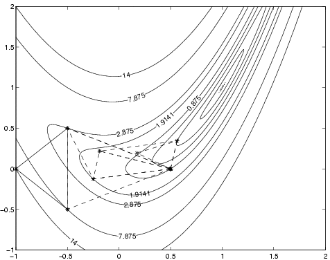
• The contour plot, if required.

To the input form