A mimimum of theory

All methods for nonlinear optimization which are available here use the same model, namely

$$\begin{eqnarray*} \mbox{NLO:} & & \\ f(x) & \stackrel{!}{=}& \min_{x} \\ \m... ...the constraints} & & \\ h(x) & = & 0 \\ g(x) & \geq & 0 \end{eqnarray*}$$

Here $f$ is a real valued scalar function, the ''objective function'', and $h$ and $g$ are two real valued vector functions. Inequalities involving vectors are to be understood componentwise. The vector $x$ has $n$ components. $h$ will have $p, p < n$ components, otherwise the problem will reduce to solving $h(x)=0$ under the additional requirements which will be explained shortly, but $g$ can have any number $m \geq 0$ of components. Of course $h$ or $g$ may also be missing in the problem, we deal with this as counting them with zero components. In the input forms the dimensions are named n, nh and ng respectively. The inequality constraints also comprise bounds on the variables, i.e. a bound

$$1 \leq x_2 \leq 4$$

must be transformed into two components of $g$ as

$$x_2 - 1 \mbox{and} 4-x_2$$

The methods which are implemented here all assume that the three functions $f, g, h$ are two times continuously differentiable, but second order derivatives are never used. We dispense you from providing the gradients, this is done here by a tool known as ''automatic differentiation''.

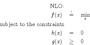
Silently we assume that points satisfying the constraints exist. It is good advise that a user makes every possible effort to find as his initial guess for a solution a $x_0$ which satisfies the constraints or at least comes near to do so, since in the nonlinear case it is quite easy to devise examples there none of the methods known will succeed from a bad $x_0$, although a well behaved solution exists. In the codes infeasibility of the problem will be reported as a failure in reducing the infeasibility below a user defined bound.

The formulation above suggests that we search for the globally best value of $x$ on the whole set described by the constraints, and indeed a typical user will hope for this. There are known methods for this, known as deterministic global optimizers, but they are presently limited to rather small dimensions and extremely cumbersome.

Practically we here are only able to identify so called first order stationary points (also known as ''Kuhn-Tucker points''). Even the characterization of these stationary points (from your calculus course you will know the condition $\nabla f(x) = 0$ for the unconstrained case) requires additional conditions. We present here only the two practically important ones, (although weaker conditions exist), namely

LICQ	linear independence condition	$(\nabla h, \nabla g_{\cal A})(x)$ has maximal rank
MFCQ	Mangasarian-Fromowitz condition	$\nabla h(x)$ has full rank and
		$\exists z \in \mathchoice{\mbox{\sf I\hspace{-0.47em} R}}{\mbox{\sf I\hs... ...hspace{-0.47em} R}}^n : \nabla h(x)^Tz = 0 , \nabla g_{\cal A}(x)^T z > 0$

In these conditions ${\cal A}$ is the index set of those $g_i(x)$ which are at their lower bound, i.e. $g_i(x) = 0$. This is the so called ''active set'' and the identification of this makes the main trouble, as you will see soon.

The notation $\nabla v$ for a vector function of $p$ components means a matrix obtained by writing the gradients of the components of $v$ (which have $n$ components themselves) side by side, i.e. a $n \times p$ matrix, the transposed Jacobian.

The direction $z$ in MFCQ is one which moves $x$ along $x+\tau z$ towards strong feasibility with respect to the active inequalities and deteriorates the equalities at most of second order in $\tau$. The MFCQ is equivalent to

$$\mbox{PLU, positive linear independence:}$$

$$(\nabla h(x))u + (\nabla g_{\cal A}(x))v = 0 \mbox{ and } v \geq 0 \Rightarrow u = 0 v = 0 .$$

In the characterization theorem one of these conditions is assumed at the solution, but in algorithmic development they are assumed to hold globally, for all $x$. Hence you never should complain on failures of a code if you give it a problem with nonlinear equality constraints which have linearly dependent gradients. For the inequalities MFCQ is more handy and there are methods which work with this one successfully.

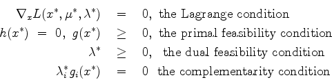
Now here comes the characterization theorem:
If $x^*$ is a local solution of NLO and either LICQ or MFCQ hold, then there exists so called multipliers $\mu^*$ and $\lambda^*$, such that the following holds:

$$\begin{eqnarray*} \nabla_x L(x^*,\mu^*,\lambda^*) &=& 0 , \mbox{ the Lagran... ...^* g_i(x^*) & = & 0 \mbox{ the complementarity condition } \end{eqnarray*}$$

The values of these four conditions are reported in the output of the codes which you can use here. The function $L$ is the so called ''Lagrange''-function of the problem and defined as

$$L(x,\mu,\lambda) = f(x) -\mu^T h(x) - \lambda^T g(x)$$

or in index notation

$$L(x,\mu,\lambda) = f(x)-\sum_{i=1}^p \mu_i h_i(x) - \sum_{j=1}^m \lambda_j g_j(x) .$$

Now if no inequality constraints would be present you can see that the identification of a Kuhn-Tucker point reduces to a (nonlinear) system of equations in $x$ and $\mu$, for which easier methods exist in another chapter. The presence of the inequalities gives the problem NLO a combinatorial character. Observe that in $L$ we deal with $\mu$ and $\lambda$ as independent variables. You will find this view back in the codes here. Sometimes all variables are considered as independent, sometimes the primal variable $x$ and sometimes the dual variables $\mu$ and $\lambda$ are the driving forces.

If LICQ holds, then the multipliers belonging to a local solution point $x^*$ are unique. They may be obtained solving the formally overdetermined system

$$\vert\vert\nabla f(x^*) - \nabla h(x^*) \mu - \nabla g_{\ca... ... \lambda \vert\vert \ \stackrel{!}{=} \min_{\mu, \lambda}$$

and with an arbitrary $x$ as guess for $x^*$ and ${\cal A}$ as a guess for the correct binding set we may use this problem (which now will not be solvable with minimum value 0) for defining approximate values for them. This technique is used in some of the algorithms presented here. The multipliers obtained this way are known as the ''least squares multipliers''.

LICQ is a very strong condition. On the other side one sees the importance of MFCQ from the fact, that the set of possible multipliers in the Kuhn-Tucker conditions is bounded if and only if MFCQ holds. Once more a warning concerning equality constraints with linearly dependent gradients.

The Kuhn-Tucker conditions are sufficient optimality conditions if the problem is convex, i.e. $f$ is convex, all the components $g_i$ of $g$ are concave and $h$ is affinely linear. In this special situation and if $f$ is even strictly convex (such that the minimizer is unique) and there exists a feasible point with $g_i(x) > 0$ for all nonlinear $g_i$ (this is the so called Slater condition) the solution of the problem NLO can be obtained by a problem of much simpler structure, namely

$$\max_{\lambda \geq 0, \mu}( \min_{x} L(x,\mu, \lambda) )$$

such that unconstrained minimization with respect to $x$ (for given $\mu, \lambda$ ) followed by a bound constrained maximization step with respect to $\mu, \lambda$ can be used as a solution process. This is used in the so called ''dual solvers'' and also in the ''augmented Lagrangian method''.

For the nonconvex case there exist local optimality criteria. We cite here only the simplest version, in which the so called ''strict complementarity condition''

$$\lambda_i^* + g_i(x^*) > 0 \quad i=1,\ldots,m$$

plays an important role. This condition has also an important practical impact: minimization of $f$ without considering an active constraint drives you out of the feasible domain. This optimality is known as ''strong second order sufficiency condition'' and reads as follows:
If a triple $(x^*,\mu^*,\lambda^*)$ satisfies the Kuhn-Tucker conditions and in addition there holds the LICQ condition, the strict complementarity condition and the matrix

$$H^* = \nabla^2_{x} L(x^*,\mu^*,\lambda^*)$$

is positive definite on the null space of the gradients of active constraints, i.e.

$$z \not = 0, \nabla h(x^*)^Tz = 0, \nabla g_{\cal A}(x^*)^Tz = 0 \Rightarrow z^TH^*z > 0 ,$$

then $x^*$ is a strict local minimizer of NLO.

This positivity condition can be reduced to a simple positive definiteness check for the so called ''projected Hessian'': if $Q$ is an orthonormal basis of the null space of the matrix $(\nabla h(x^*),\nabla g_{\cal A}(x^*))$ then one simply has to test $Q^TH^*Q$ for positive definiteness, for example by trying its Cholesky decomposition. In the prepared testcases the two extreme eigenvalues of $Q^TH^*Q$ are reported.