Test examples of boundary value problems

1 Example1

This is a linear case satisfying strong uniqueness and smoothness conditions. The problem is originally a scalar second order problem:

y " = \frac{2 y}{(1 + x)^{2}}, y (0) = 1, y (1) = \frac{1}{2}

with the unique and arbitrarily smooth solution

y (x) = \frac{1}{1 + x} .

This is transformed into the first order system

\begin{matrix} y_{1}' & = & y_{2}, \\ y_{2}' & = & \frac{2 y_{1}}{(1 + x)^{2}} \end{matrix}

and we use the true boundary values as initial guess:

y_{1} (0) = 1, y_{2} (0) = - 1.0, y_{1} (1) = 0.5, y_{2} (1) = - 0.25 .

Because of this and the linearity in

y

Newton's method finds the true solution in one step (you see only the computed solution on the plot), but in order to detect this it takes a second step.

2 Example2

This is a nonlinear, uniquely solvable, but sensitive case. This is also a scalar second order problem originally,

y " = (y')^{2}, y (- 1) = 0, y (1) = \log (10)

with the unique and arbitrarily smooth solution

y (x) = - \log (\frac{11}{20} - \frac{9}{20} x)

This is again transformed into a first order system

\begin{matrix} y_{1}' & = & y_{2} \\ y_{2}' & = & (y_{2})^{2} \end{matrix}

If with only one interval the initial value problem would be solved with an initial slope

\geq 0.5

then a singularity of the solution occurs inside

[- 1, 1]

and the integrator could not finish his job. We take here 4 subintervals of length 0.5 and use the values of the linear interpolant of the boundary values as initial guesses. The first integration hence yields a discontinuous solution, but Newton's method converges fast and without trouble.

3 Example3

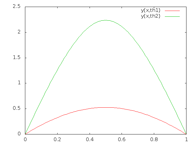
This is a nonlinear nonuniquely solvable case with two smooth solutions. This is also a scalar second order bondary value problem

y " = - \exp (y + 1), y (0) = 0, y (1) = 0

nonlinear as the second example, but this one is not uniquely solvable. It has two solutions

y (x) = - 2 \log (\frac{\cosh ((x - \frac{1}{2}) \frac{θ}{2})}{\cosh (\frac{θ}{4})})

where

θ

is one of the two solutions of

θ = \sqrt{2 e} \cosh (\frac{θ}{4}) .

These values are

θ = 3.036231848196573

for the lower and

θ = 7.135005531636586

for the upper solution.

Again this is transformed to a first order system. We use

m = 2

(simple shooting) and the zero function as the default initial solution. From this Newton's method converges quickly against the lower solution.

4 Example4

The following is taken from J. Stoer and R. Bulirsch: "Introduction to Numerical Mathematics", volume II, 1973, pages 180-186. This is the famous reentry problem of an APOLLO like space vehicle, solved here under simplifying assumptions: earth is a sphere with radius

R

. The variables describing the flight are speed

v

, the angle

γ

between the flight's curve tangent and the tangent to the sphere at the current projection point of the vehicle position on the sphere, the normalized heigth

ξ

= distance from earth divided by

R

. The equations read

\begin{matrix} \overset{\cdot}{v} & = & V (t, v, γ, ξ, u) = - \frac{S ρ v^{2}}{2 m} C_{w} (u) - \frac{g \sin (γ)}{(1 + ξ)^{2}} \\ \overset{\cdot}{γ} & = & Γ (t, v, γ, ξ, u) = \frac{S ρ v}{2 m} C_{A} (u) + \frac{v \cos (γ)}{R (1 + ξ)} - \frac{g \cos (γ)}{v (1 + ξ)^{2}} \\ \overset{\cdot}{ξ} & = & Ξ (t, v, γ, ξ, u) = \frac{v \sin (γ)}{R} \end{matrix}

Here

ρ = ρ_{0} \exp (- β R ξ)

is the density of the atmosphere,

β

a constant,

m

mass and

S

the frontal area, and

g

earth acceleration. The physical parameters are

10^{5}

feet for space and second for time. Values are

R = 209, β = 4.26, ρ_{0} = 0.002704, g = 0.00032172, S / m = 53200 .

The coefficients

C_{A} (u) = 0.6 \sin (u), C_{W} (u) = 1.174 - \cos (u)

(aerodnamical lift and aerodynamical resistance coefficient) describe the influence of a control function

u

which serves for changing

S

during flight (brake flaps). The aim of this control is the minimization of the total heating of the vehicle during the manoeuvre which is given by

J = \int_{0}^{T} {10 v^{3} \sqrt{ρ}} d t

The endtime

T

is free. There are initial and end conditions:

v (0) = 0.36, γ (0) = 8.1 π / 180, ξ (0) = 4 / R

and

v (T) = 0.27, γ (T) = 0, ξ (T) = 2.5 .

From variational analysis it follows that this free endtime minimization problem in function space can be solved by requiring

H_{t = T} = 0

where

H

is the Hamiltonian function

H (t, v, γ, ξ, u) = 10 v^{3} \sqrt{ρ} + λ_{v} V (t, v, γ, ξ, u) + λ_{γ} Γ (t, v, γ, ξ, u) + λ_{ξ} Ξ (t, v, γ, ξ, u) .

λ_{v}, λ_{γ}, λ_{ξ}

themselves, the multipliers for the constraints on

v, γ, ξ

, are again functions, defined by the differential equations

\begin{matrix} \overset{\cdot}{λ_{v}} & = & - \frac{\partial H}{\partial v} \\ \overset{\cdot}{λ_{γ}} & = & - \frac{\partial H}{\partial γ} \\ \overset{\cdot}{λ_{ξ}} & = & - \frac{\partial H}{\partial ξ} \end{matrix}

The control

u

is given by

\sin (u) = - \frac{0.6 λ_{γ}}{α}, \cos (u) = \frac{- 0.9 v λ_{v}}{α}, α = \sqrt{(0.6 λ_{γ})^{2} + (0.9 v λ_{v})^{2}} .

The indices in the vector solution

y

correspond to the appearance of the variables here:

y_{1}

is speed,

y_{2}

is angle,

y_{3}

is normalized height,

y_{4}, y_{5}, y_{6}

are the three multipliers for the constraints and

y_{7}

represents the endtime with the ode

\overset{\cdot}{y_{7}} = 0 .

This is a highly sensitive problem. We use here the initial values given by Deuflhard and coworkers. You may play with the parameter tol but changing the initial values is discouraged.

File translated from T_EX by T_TM Unregistered, version 4.03.
On 20 Jun 2016, 17:59.